
 資料結構
資料結構 網路
網路 關係型資料庫管理系統 (RDBMS)
 作業系統
作業系統 Java
Java iOS
iOS HTML
HTML CSS
CSS Android
 Python
 C語言程式設計
 C++
C++ C#
C# MongoDB
 MySQL
MySQL Javascript
 PHP
PHP使用PyTorch實現深度自編碼器進行影像重建
機器學習是人工智慧的一個分支,它涉及開發能夠使計算機從輸入資料中學習並做出決策或預測的統計模型和演算法,而無需硬編碼。它涉及使用大型資料集訓練機器學習演算法,以便機器能夠識別資料中的模式和關係。
什麼是自編碼器?
具有自編碼器的神經網路架構用於無監督學習任務。它由編碼器和解碼器網路組成,這些網路經過訓練可以重建輸入資料,方法是將其壓縮成低維表示(編碼),然後對其進行解碼以恢復其原始形式。
為了鼓勵網路學習資料的有價值的特徵或表示,目標是最小化輸入和輸出之間的重建誤差。自編碼器的突出應用包括資料壓縮、影像去噪和異常檢測。這減少了與資料傳輸相關的許多工作和成本。
在本文中,我們將探討如何使用PyTorch的深度自編碼器進行影像重建。這個深度學習模型將使用MNIST手寫數字進行訓練,在學習輸入影像的表示後,它將重建數字影像。一個基本的自編碼器包含兩個主要功能:
編碼器
解碼器
編碼器接收輸入,並透過一系列層將高維資料轉換為相同值的潛在低維表示。解碼器使用此潛在表示,使用Python庫torch、PyTorch工作流程中的torchvision庫以及numpy和matplotlib等通用庫來生成重建資料。
演算法
匯入所有必需的庫。
初始化將應用於獲得的資料集的每個條目的轉換操作。
由於Pytorch需要張量才能執行,因此我們首先將每個專案轉換為張量並對其進行歸一化,以保持畫素值在0到1之間的範圍。
使用torchvision.datasets程式下載資料集,並分別將其儲存在./MNIST/train和./MNIST/test資料夾中,用於訓練集和測試集。
為了加快學習速度,將這些資料集轉換為批次大小等於64的資料載入器。
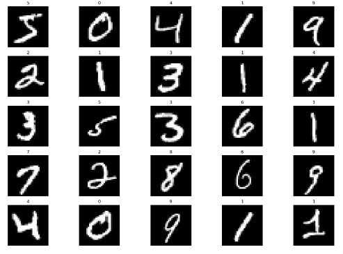
隨機列印集合中的25張照片,以便我們更好地理解正在處理的資訊。
步驟1:初始化
此步驟涉及匯入所有必要的庫,例如numpy、matplotlib、pytorch和torchvision。
語法
torchvision.transforms.ToTensor():
將輸入影像(以PIL或numpy格式)轉換為PyTorch張量格式。此轉換還將畫素強度從[0, 255]範圍縮放為[0, 1]。
torchvision.transforms.Normalize(mean, std)
使用均值和標準差值對輸入影像張量進行歸一化。此轉換有助於提高深度學習模型在訓練期間的收斂速度。均值和標準差值通常是從訓練資料集中計算出來的。
torchvision.transforms.Compose(transforms)
允許將多個影像轉換連結到單個物件中。此物件可以傳遞給PyTorch Dataset物件,以便在訓練或推理期間動態應用轉換。
示例
#importing modules
import numpy as np
import matplotlib.pyplot as plt
import torch
from torchvision import datasets, transforms
plt.rcParams['figure.figsize'] = 15, 10

# Initialize the transform operation
transform = torchvision.transforms.Compose([
   torchvision.transforms.ToTensor(),
   torchvision.transforms.Normalize((0.5), (0.5))
])

# Download the inbuilt MNIST data
train_dataset = torchvision.datasets.MNIST(
   root="./MNIST/train", train=True,
   transform=torchvision.transforms.ToTensor(),
   download=True)
test_dataset = torchvision.datasets.MNIST(
   root="./MNIST/test", train=False,
   transform=torchvision.transforms.ToTensor(),
   download=True)
輸出
步驟2:初始化自編碼器
我們首先初始化Autoencoder類,它是torch.nn.Module的子類。由於這為我們抽象了許多樣板程式碼,因此我們現在可以專注於建立我們的模型架構,如下所示:
語法
torch.nn.Linear()
一個將線性變換應用於輸入張量的模組。
my_linear_layer = nn.Linear(in_features, out_features, bias=True)
torch.nn.ReLU()
一個將修正線性單元 (ReLU) 函式應用於輸入張量的啟用函式。
torch.nn.Sigmoid()
一個將sigmoid函式應用於輸入張量的啟用函式。
示例
#Creating the autoencoder classes
class Autoencoder(torch.nn.Module):
   def __init__(self):
      super().__init__()
      self.encoder=torch.nn.Sequential(
         torch.nn.Linear(28*28,128), #N, 784 -> 128
         torch.nn.ReLU(),
         torch.nn.Linear(128,64),
         torch.nn.ReLU(),
         torch.nn.Linear(64,12),
         torch.nn.ReLU(),
         torch.nn.Linear(12,3), # --> N, 3
         torch.nn.ReLU()
      )

      self.decoder=torch.nn.Sequential(
         torch.nn.Linear(3,12), #N, 3 -> 12
         torch.nn.ReLU(),
         torch.nn.Linear(12,64),
         torch.nn.ReLU(),
         torch.nn.Linear(64,128),
         torch.nn.ReLU(),
         torch.nn.Linear(128,28*28), # --> N, 28*28
         torch.nn.Sigmoid()
      )

   def forward(self,x):
      encoded=self.encoder(x)
      decoded = self.decoder(encoded)
      return decoded

# Instantiating the model and hyperparameters
model = Autoencoder()
criterion = torch.nn.MSELoss()
num_epochs = 10
optimizer = torch.optim.Adam(model.parameters(), lr=1e-3)
步驟3:建立訓練迴圈
我們正在訓練一個自編碼器模型來學習影像的壓縮表示。訓練迴圈總共遍歷資料集10次。
為每批影像迭代計算模型的輸出。
然後計算輸出影像和原始影像之間的質量差異。
它平均每批的損失,並存儲每個 epoch 的影像及其輸出。
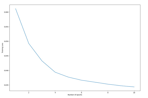
迴圈完成後,我們繪製訓練損失,以幫助理解訓練過程。
該圖顯示損失隨著每個 epoch 的推移而降低,這表明模型正在學習新的資訊,並且訓練過程是成功的。
訓練迴圈訓練自編碼器模型,透過最小化輸出影像和原始影像之間的損失來學習影像的壓縮表示。損失隨著每個 epoch 的增加而減少,表明訓練成功。
示例
# Create empty list to store the training loss
train_loss = []
# Create empty dictionary to store the images and their reconstructed outputs
outputs = {}
# Loop through each epoch
for epoch in range(num_epochs):
   # Initialize variable for storing the running loss
   running_loss = 0
   # Loop through each batch in the training data
   for batch in train_loader:

      # Load the images and their labels
      img, _ = batch
      # Flatten the images into a 1D tensor
      img = img.view(img.size(0), -1)
      # Generate the output for the autoencoder model
      out = model(img)
      # Calculate the loss between the input and output images
      loss = criterion(out, img)
      # Reset the gradients
      optimizer.zero_grad()
      # Compute the gradients
      loss.backward()
      # Update the weights
      optimizer.step()
      # Increment the running loss by the batch loss
      running_loss += loss.item()
   # Calculate the average running loss over the entire dataset
   running_loss /= len(train_loader)
   # Add the running loss to the list of training losses
   train_loss.append(running_loss)
   # Store the input and output images for the last batch
   outputs[epoch+1] = {'input': img, 'output': out}

# Plot the training loss over epochs
plt.plot(range(1, num_epochs+1), train_loss)
plt.xlabel("Number of epochs")
plt.ylabel("Training Loss")
plt.show()
輸出
步驟4:視覺化
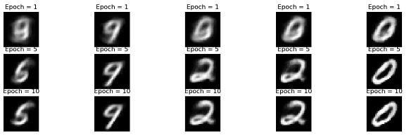
此程式碼繪製訓練好的自編碼器模型的原始影像和重建影像。變數outputs包含有關模型輸出的資料,例如重建影像和在不同訓練 epoch 中記錄的損失值。使用list_epochs變數來繪製特定 epoch 的重建影像。
該程式繪製給定 epoch 的最後一批中的前五張重建影像。
示例
# Plot the re-constructed images
# Initializing the counter
count = 1
# Plotting the reconstructed images
list_epochs = [1, 5, 10]

# Iterate over specified epochs
for val in list_epochs:

   # Extract recorded information
   temp = outputs[val]['out'].detach().numpy()
   title_text = f"Epoch = {val}"

   # Plot first 5 images of the last batch
   for idx in range(5):
      plt.subplot(7, 5, count)
      plt.title(title_text)
      plt.imshow(temp[idx].reshape(28,28), cmap= 'gray')
      plt.axis('off')

      # Increment the count
      count+=1

# Plot of the original images

# Iterating over first five
# images of the last batch
for idx in range(5):

   # Obtaining image from the dictionary
   val = outputs[10]['img']

   # Plotting image
   plt.subplot(7,5,count)
   plt.imshow(val[idx].reshape(28, 28),
               cmap = 'gray')
   plt.title("Original Image")
   plt.axis('off')

   # Increment the count
   count+=1

plt.tight_layout()
plt.show()
輸出
步驟5:測試集效能評估
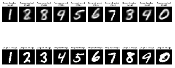
此程式碼是關於如何在測試集上評估訓練好的自編碼器模型的效能的示例。
程式碼根據對重建影像的視覺檢查得出結論,自編碼器模型在測試集上表現良好。如果模型在測試集上表現良好,則它很可能在新資料上表現良好。
示例
outputs = {}

# Extract the last batch dataset
img, _ = list(test_loader)[-1]

img = img.reshape(-1, 28 * 28)

#Generating output
out = model(img)

# Storing results in the dictionary
outputs['img'] = img
outputs['out'] = out

# Initialize subplot count
count = 1
val = outputs['out'].detach().numpy()

# Plot first 10 images of the batch
for idx in range(10):
   plt.subplot(2, 10, count)
   plt.title("Reconstructed \n image")
   plt.imshow(val[idx].reshape(28, 28), cmap='gray')
   plt.axis('off')

   # Increment subplot count
   count += 1
# Plotting original images
# Plotting first 10 images
for idx in range(10):
   val = outputs['img']
   plt.subplot(2, 10, count)
   plt.imshow(val[idx].reshape(28, 28), cmap='gray')
   plt.title("Original Image")
   plt.axis('off')
   count += 1

plt.tight_layout()
plt.show()
輸出
結論
總之,自編碼器是強大的神經網路,可以應用於許多不同的任務,包括資料壓縮、異常檢測和影像生成。TensorFlow、Keras和PyTorch是一些使自編碼器開發簡單的Python工具。透過理解架構和調整引數,可以構建非常強大的自編碼器模型。隨著機器學習領域的進步,自編碼器很可能繼續成為各種應用的有用工具。

瀏覽量:585
